Data Comparison

Excel 2013

Do you need to compare two lists of data in Excel and find differences?

How can you do it quickly?

Compare both lists with a single formula

First copy your original data into a worksheet.
Copy the new data into the same worksheet, next to the original data.
Sort both lists into the same order.

Now you are ready to start comparing the lists.

We are going to use the AND function to do the comparison.
The first step is to compare all the data in a single step. If there are no differences then there is no need to run further comparisons.

The formula needs be entered as an Array formula using the key combination Ctrl + Shift + Enter instead of just Enter.

=AND(A3:B6=D3:E6)

If the formula returns TRUE then the two lists match. If it returns FALSE then something doesn’t match.

Compare each cell

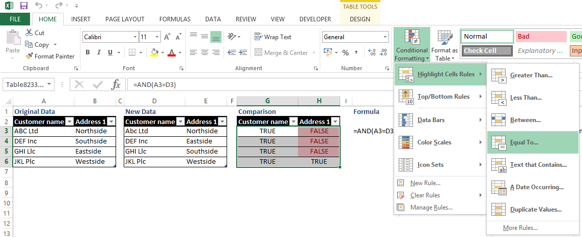
To continue the analysis, create an area to the right of the two lists to enter comparison formulas.

We will continue to use the AND function to compare the data, but this time on a cell by cell basis rather than in an array.

=AND(A3=D3)

Enter this formula into the top left cell of the comparison range and then copy it across the whole comparison range.

If the cells match then the formula returns TRUE otherwise it returns FALSE.

Ignore spacing differences

Some data will have extra spaces or use spaces for padding. This will cause the formula to return FALSE.

In the screenshot, an extra space has been added to the end of the address in the first row. This isn’t visible unless you edit the cell.

If you consider the data as matching regardless of the spacing, the AND function can be combined with CLEAN and TRIM functions.

CLEAN removes non-printable characters.
TRIM removes any leading or trailing spaces as well as reducing all internal spacing to single spaces.

=AND(TRIM(CLEAN(A3))=TRIM(CLEAN(D3)))

Conditional Formatting

If the lists contain a large amount of data, it is difficult to immediately see cells marked as FALSE. Conditional formatting can be used to highlight cells containing the FALSE value.

Select the comparison data range.
Navigate to the Home menu tab and click on the Conditional Formatting icon.
Select Highlight Cell Rules and Equal To.

Type FALSE into the box and click on the OK button.

Any cells in the comparison range containing FALSE will be highlighted.

Compare case

The one thing that the AND function ignores when it does the comparison is the case of the cell values.
So ABC Ltd = Abc Ltd always evaluates to TRUE.

If you need to compare the case of the cells then you need to use the EXACT function

=EXACT(TRIM(CLEAN(A3)),TRIM(CLEAN(D3)))